Multi-Label Audio Classification Using Spectrogram Images

Introduction

This blog post covers my work on Freesound Audio Tagging 2019, a past Kaggle competition involving multi-label audio tagging with 80 categories (e.g., applause, bicycle bell, chink and clink, keys jangling). The goal is to determine which categories a particular sound clip belongs to.

Notice that this is a multi-label, not multi-class, problem. In multi-label classification, a sound clip can have one or more categories that it belongs to. In multi-class classification, a sound clip can only belong to one class out of multiple classes.

I’ll discuss my approach — converting audio files to spectrogram images and treating this as a computer vision classification problem — and data processing steps as well as training results in the following sections. My motivation for working on this competition was to learn how to handle audio data and multi-label classification in PyTorch, which were new to me.

Dataset

This competition provided two different training datasets: a “curated” set and a “noisy” set. My work only focuses on the curated set, a smaller but more reliable dataset that was manually labeled by humans. It has 4970 audio clips, about 75 clips per category, and 10.5 hours in total duration. Clips are 0.3 to 30 seconds long.

Let’s listen to a few audio clips.

This is a gong:

This is a bass drum:

This is a bus:

I converted all of the audio files to spectrogram images to take advantage of existing pre-trained computer vision models. Note that when this competition was active three years ago, pre-trained models were not allowed, so competitors had to train their models from scratch.

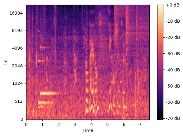
Spectrograms are visual representations of sound, with frequency on the y-axis and time on the x-axis. Different types of noises have different features, so it is reasonable to expect that we could identify a particular category of sound by its spectrogram. In particular, we use mel spectrograms, where the frequency scale is no longer linear so it better models human hearing perception.

Processing Using Librosa

I used a Python audio library called librosa to visualize audio waveforms and spectrograms. Below, I’ll go over some of its basic functions using the “bus” example clip from earlier.

Load the audio file:

import librosa

y, sr = librosa.load('9a7c3b2c.wav', sr=None)

By default, librosa.load automatically resamples the audio to 22,050 Hz; to avoid this, set sr=None so that we can use the native sampling rate of 44,100 Hz. Additionally, librosa.load will normalize the data so that values are between -1.0 and +1.0, and will convert stereo (2 channels) to mono (1 channel).

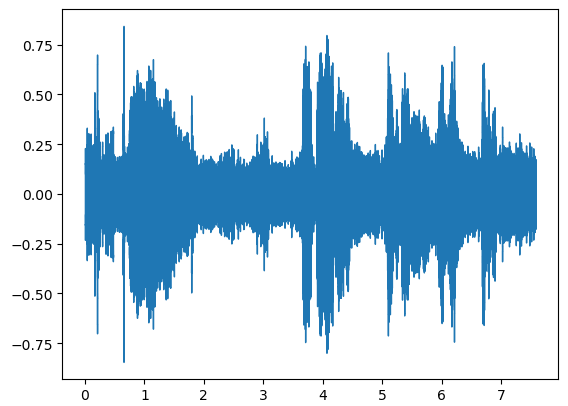
View the audio file’s waveform:

import librosa.display

librosa.display.waveshow(y, sr=sr)

Generate a mel spectrogram:

import matplotlib.pyplot as plt

S = librosa.feature.melspectrogram(y=y, sr=sr, n_fft=2048, hop_length=512, n_mels=128, fmin=20, fmax=8300)
S_DB = librosa.power_to_db(S, ref=np.max)
librosa.display.specshow(S_DB, sr=sr, x_axis='time', y_axis='mel');
plt.colorbar(format='%+2.0f dB');

In the librosa.feature.melspectrogram function above:

• n_fft is the length of the FFT window; we are using 2048 samples for each window
• hop_length is the number of samples between successive frames; we are moving the window by skipping 512 samples to get to the next time frame
• n_mels is the number of Mel bands/filters to generate; the height of our spectrogram image is 128
• fmin and fmax are the minimum and maximum frequencies

To put it all together, here’s the code to convert all of our curated training set’s audio files to PNG image files (took ~20 minutes to run on my CPU):

import pandas as pd
import os
import librosa
import librosa.display
import matplotlib.pyplot as plt
import numpy as np

# Read in the curated training set CSV file as a DataFrame
data_dir = 'freesound-audio-tagging-2019/'
train_cur = pd.read_csv(data_dir + 'train_curated.csv', low_memory=False)

# Create the directory holding all images
images_dir = data_dir + 'train_curated_images/'
os.mkdir(images_dir)

# Go through each row
for i in train_cur.index:

    # Load and convert to a mel spectrogram
    file_i = train_cur['fname'].loc[i]
    y, sr = librosa.load(data_dir+'train_curated'+'/'+file_i, sr=None)
    mel = librosa.feature.melspectrogram(y=y, sr=sr, n_fft=2560, hop_length=512, n_mels=128, fmin=20, fmax=22050)
    mel_db = librosa.power_to_db(mel, ref=np.max)

    # Convert the mel spectrogram to an image, and save
    fig, ax = plt.subplots()
    ax.axes.get_xaxis().set_visible(False)
    ax.axes.get_yaxis().set_visible(False)
    ax.set_frame_on(False)
    librosa.display.specshow(mel_db, sr=sr)
    plt.savefig(images_dir+'/'+file_i[:-3]+'png', dpi=400, bbox_inches='tight', pad_inches=0)
    plt.close('all')

And that’s it! Now we have the images we need to turn this audio classification problem into a computer vision one.

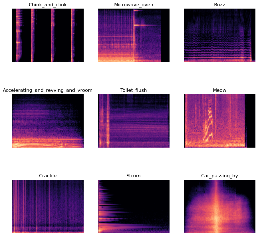
Here’s a collage of some mel spectrograms, alongside their label:

Multi-Hot-Encoding

We need to convert our training DataFrame (which contains our labels aka the ground truth) to a multi-hot-encoded format of 0s and 1s, which we’ll feed into our model.

Right now it looks like this, which isn’t ideal:

87e74683.png	Skateboard
c99f7507.png	Gong
771f6c75.png	Female_singing
3f53058e.png	Acoustic_guitar,Strum
97f7cd56.png	Skateboard
...

Instead, we want there to be 80 columns representing 80 categories, with values of 0 or 1 denoting whether the spectrogram doesn’t or does belong to a particular category, respectively.

Perform multi-hot-encoding using scikit-learn’s MultiLabelBinarizer and save to file:

from sklearn.preprocessing import MultiLabelBinarizer

# Create an iterable of iterables, as required by scikit-learn
y = [f.split(',') for f in train_cur['labels']]

# Get multi-hot-encoded labels
mlb = MultiLabelBinarizer()
labels_mlb = mlb.fit_transform(y)

# Save to file
train_cur[mlb.classes_] = labels_mlb
train_cur = train_cur.drop(labels='labels', axis=1)
train_cur.to_csv('train_curated_image_labels.csv', index=False)

All done! You can view the total number of samples using len(labels_mlb), and view the number of categories per sample using len(labels_mlb[0]).

Print a list of all categories:

mlb.classes_

array(['Accelerating_and_revving_and_vroom', 'Accordion',
   'Acoustic_guitar', 'Applause', 'Bark', 'Bass_drum', 'Bass_guitar',
   'Bathtub_(filling_or_washing)', 'Bicycle_bell',
   'Burping_and_eructation', 'Bus', 'Buzz', 'Car_passing_by',
   'Cheering', 'Chewing_and_mastication',
   'Child_speech_and_kid_speaking', 'Chink_and_clink',
   'Chirp_and_tweet', 'Church_bell', 'Clapping', 'Computer_keyboard',
   'Crackle', 'Cricket', 'Crowd', 'Cupboard_open_or_close',
   'Cutlery_and_silverware', 'Dishes_and_pots_and_pans',
   'Drawer_open_or_close', 'Drip', 'Electric_guitar', 'Fart',
   'Female_singing', 'Female_speech_and_woman_speaking',
   'Fill_(with_liquid)', 'Finger_snapping', 'Frying_(food)', 'Gasp',
   'Glockenspiel', 'Gong', 'Gurgling', 'Harmonica', 'Hi-hat', 'Hiss',
   'Keys_jangling', 'Knock', 'Male_singing',
   'Male_speech_and_man_speaking', 'Marimba_and_xylophone',
   'Mechanical_fan', 'Meow', 'Microwave_oven', 'Motorcycle',
   'Printer', 'Purr', 'Race_car_and_auto_racing', 'Raindrop', 'Run',
   'Scissors', 'Screaming', 'Shatter', 'Sigh',
   'Sink_(filling_or_washing)', 'Skateboard', 'Slam', 'Sneeze',
   'Squeak', 'Stream', 'Strum', 'Tap', 'Tick-tock', 'Toilet_flush',
   'Traffic_noise_and_roadway_noise', 'Trickle_and_dribble',
   'Walk_and_footsteps', 'Water_tap_and_faucet', 'Waves_and_surf',
   'Whispering', 'Writing', 'Yell', 'Zipper_(clothing)'], dtype=object)

Training/Validation Split

The last thing we want to do before we can train a model is to split our provided data into training and validation sets.

This can be straightforwardly done with scikit-learn’s train_test_split:

import pandas as pd
from sklearn.model_selection import train_test_split
import numpy as np

all_data = pd.read_csv('train_curated_image_labels.csv')

train_idx, valid_idx = train_test_split(np.arange(len(all_data)), test_size=0.25, random_state=42)
train_df = all_data.iloc[train_idx]
valid_df = all_data.iloc[valid_idx]

train_df.to_csv('train_curated_image_trainset.csv', index=False)
valid_df.to_csv('train_curated_image_validset.csv', index=False)

Great! We have our training and validation sets clearly marked in separate CSV files.

Training

Training was done in PyTorch. The training and validation sets are loaded in using a Dataset class and DataLoader:

class MultiLabelDataset(Dataset):
    def __init__(self, annotations_file, img_dir, transform=None, target_transform=None):
        self.img_labels = pd.read_csv(annotations_file, low_memory=False)
        self.img_dir = img_dir
        self.transform = transform
        self.target_transform = target_transform
    def __len__(self):
        return len(self.img_labels)
    def __getitem__(self, idx):
        img_path = os.path.join(self.img_dir, self.img_labels.iloc[idx, 0])
        image = read_image(img_path, mode=ImageReadMode.RGB)
        labels = self.img_labels.iloc[idx, 1:].to_numpy()
        if self.transform:
            image = self.transform(image)
        if self.target_transform:
            labels = self.target_transform(labels)
        return image, labels.astype(float)

def load_multilabel_images(img_dir, train_csv, valid_csv, transforms, batch_size=32, num_workers=0):
    train_data = MultiLabelDataset(train_csv, img_dir, transform=transforms['train'])
    valid_data = MultiLabelDataset(valid_csv, img_dir, transform=transforms['valid'])
    train_dataloader = DataLoader(
        train_data,
        batch_size=batch_size,
        shuffle=True,
        num_workers=num_workers,
        pin_memory=True,
    )
    valid_dataloader = DataLoader(
        valid_data,
        batch_size=batch_size,
        shuffle=True,
        num_workers=num_workers,
        pin_memory=True,
    )
    return train_dataloader, valid_dataloader

data_dir = 'train_curated_images/'
train_csv = 'train_curated_image_trainset.csv'
valid_csv = 'train_curated_image_validset.csv'
train_dl, valid_dl = load_multilabel_images(img_dir=data_dir, train_csv=train_csv, valid_csv=valid_csv, transforms=data_transforms, batch_size=32, num_workers=0)

I used a pre-trained model called ConvNeXt Tiny, which can be instantiated thusly:

def create_convnext_tiny(out_features, device):
    weights = torchvision.models.ConvNeXt_Tiny_Weights.DEFAULT
    model = torchvision.models.convnext_tiny(weights=weights).to(device)

    for param in model.features.parameters():
        param.requires_grad = False

    model.classifier = nn.Sequential(
        torchvision.models.convnext.LayerNorm2d((768,), eps=1e-06, elementwise_affine=True),
        nn.Flatten(start_dim=1, end_dim=-1),
        nn.Linear(in_features=768, out_features=out_features, bias=True)
    ).to(device)
    
    model.name = 'ConvNeXt Tiny'
    print(f'[INFO] Created new {model.name} model.')

    return model, weights

device = 'cuda' if torch.cuda.is_available() else 'cpu'
model, weights = create_convnext_tiny(out_features=80, device=device)

I used binary cross-entropy for the loss function. I chose BCEWithLogitsLoss instead of BCELoss because the former includes a sigmoid layer and can be more numerically stable — see documentation. torch.optim.Adam was mainly used as the optimization algorithm.

Training was performed by looping through every epoch. For example, this is a function for a single training epoch:

def train_step_lrap(model, dataloader, loss_fn, optimizer, device):
    model.train()
    train_loss, train_lrap = 0, 0

    for batch, (X, y) in enumerate(dataloader):
        X, y = X.to(device), y.to(device)

        y_pred = model(X)
        loss = loss_fn(y_pred, y)
        train_loss += loss.item() 

        optimizer.zero_grad()
        loss.backward()
        optimizer.step()

        train_lrap += label_ranking_average_precision_score(y, torch.sigmoid(y_pred).detach().numpy())

    train_loss = train_loss / len(dataloader)
    train_lrap = train_lrap / len(dataloader)

    return train_loss, train_lrap

During training, I explored:

• learning rates ranging from 1e-05 to 1e-02 (this sometimes helped)
• batch sizes ranging from 8 to 128 (this sometimes helped)
• SGD optimizer (this didn’t help)
• different sets of mel spectrogram images generated using different settings (this didn’t help)
• image augmentation, including transforms such as RandomCrop, RandAugment, TrivialAugmentWide (this didn’t help)
• binarizing results to 0 or 1, using different thresholds (this didn’t help)

My general strategy was to train using a small number of epochs at a time (3 to 5), which took ~6 minutes per epoch on my CPU. I often started from a previous run’s trained model.

Results

My best model was scored as 0.52 by Kaggle, which would put me in the top 26% of the leaderboard at the time of the competition. Note that this score is an evaluation metric called the label-weighted label-ranking average precision (“lwlrap”).

An important distinction is that I used a pre-trained model, whereas the competitors at the time were not allowed to do so, according to the competition rules.