IceCube Neutrino Reconstruction Using PCA and RNNs
Introduction
IceCube is a neutrino observatory encompassing a cubic kilometer of ice in the South Pole. One of the challenges associated with neutrino research is how we can quickly and accurately determine the direction that a neutrino came from. I participated in IceCube’s machine learning competition, hosted on Kaggle, that challenged competitors to accurately process a large number of neutrino events (about 1 million events in the hidden test set) within time constraints.
My goal was to use this competition as an opportunity to gain familiarity with principal component analysis (PCA) as well as sequential models such as recurrent neural networks (RNNs).
In the sections below, I’ll cover my work on exploratory data analysis, PCA, and RNNs, and share any relevant snippets of code along the way.
Exploratory Data Analysis
Let’s first take a look at IceCube’s sensor geometry. IceCube consists of 5160 sensors, and we are provided with the x, y, and z positions of each sensor.
Read in the sensory geometry CSV file, and create a 3D scatter plot using Plotly:
sensor_geometry = pd.read_csv('/Volumes/public/Python/icecube/sensor_geometry.csv')
sensor_geometry.head()

plotly.offline.init_notebook_mode()

trace = go.Scatter3d(
    x=sensor_geometry['x'],
    y=sensor_geometry['y'],
    z=sensor_geometry['z'],
    mode='markers',
    marker={'color': sensor_geometry['sensor_id'], 'colorscale': 'Viridis', 'size': 2, 'colorbar': dict(thickness=20)}
)

layout = go.Layout(margin={'l': 0, 'r': 0, 'b': 0, 't': 0})

plot_figure = go.Figure(data=[trace], layout=layout)

plotly.offline.iplot(plot_figure)
I ran this code in a Jupyter Notebook so that the interactive plot would appear alongside the code cell. This is what it looks like:
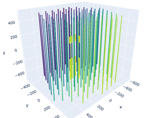
The darker colors correspond to lower sensor IDs and the lighter colors correspond to higher sensor IDs. You can see that the sensors are located along vertical “strings.”
The competition provides 131,953,924 neutrino events for our training purposes. Each neutrino event has a ground truth label (azimuth and zenith values), which specifies the direction that the neutrino came from. We have accurate labels for this dataset because this is synthetic data.
These labels are located in a train_meta.parquet file, which we’ll read in:
train_meta = pd.read_parquet('/Volumes/public/Python/icecube/train_meta.parquet')
train_meta.head()
batch_id	event_id	first_pulse_index	last_pulse_index	azimuth	    zenith
1	        24	        0	                60	                5.029555	2.087498
1	        41	        61	                111	                0.417742	1.549686
1	        59	        112	                147	                1.160466	2.401942
1	        67	        148	                289	                5.845952	0.759054
1	        72	        290	                351	                0.653719	0.939117
You can see that each row of this file corresponds to a separate neutrino event.
The data for each neutrino event are located in individual batch files (a total of 660 batch IDs) stored as parquets. Let’s open up batch_7.parquet:
train_batch_7 = pd.read_parquet('/Volumes/public/Python/icecube/train/batch_7.parquet')
train_batch_7.head()
            sensor_id	time	charge	auxiliary
event_id
19526675	288	        6004	0.575	True
19526675	3257	    6360	1.175	True
19526675	303	        6490	1.025	True
19526675	2354	    7517	0.625	True
19526675	4104	    7850	1.075	True
Reading in batch #7 takes up about 840 MB memory. We can see that there are multiple rows per event, with each row describing the sensor ID that detected a pulse. Relative time of the pulse and its charge are also provided. auxiliary is a column where False means that the pulse was fully digitized and is likely of higher quality.
Let’s take a look at the distribution of pulse charge. Plot a histogram of its distribution:
plt.hist(train_batch_7['charge'], bins=30, range=(0, 6))
plt.xlabel('Pulse Charge [photoelectrons]')
plt.ylabel('Count')
plt.show()
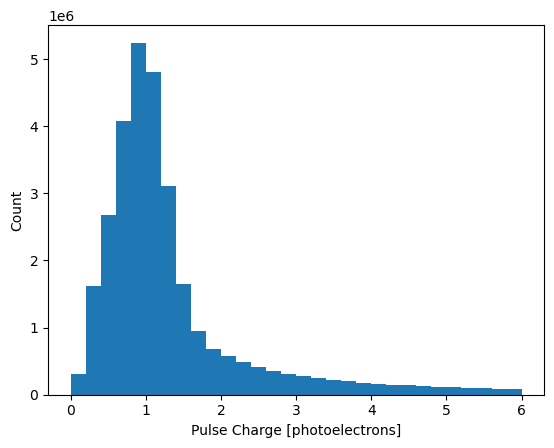
Most pulses have a charge of about 1 photoelectron.
Let’s plot any given event including the pulse-detecting sensors and a line depicting the neutrino’s direction. We’ll write a function and use Plotly again for 3D plotting. Here’s the code along with comments:
def plot_event(event_id):

    # Get pulse-detecting sensors
    sample_event = train_batch_7.loc[event_id, 'sensor_id']
    sample_sensors = pd.merge(sensor_geometry, sample_event, on='sensor_id', how='inner')

    # Convert polar coordinates (azimuth, zenith) to cartesian coordinates (x, y, z)
    azimuth = train_meta[train_meta['event_id'] == event_id]['azimuth'].squeeze()
    zenith = train_meta[train_meta['event_id'] == event_id]['zenith'].squeeze()
    r = 500
    x_line = r * np.cos(azimuth) * np.sin(zenith)
    y_line = r * np.sin(azimuth) * np.sin(zenith)
    z_line = r * np.cos(zenith)

    # Set up plotly to display in notebook mode
    plotly.offline.init_notebook_mode()

    # Create traces for each scatterplot
    trace = go.Scatter3d(
        x=sensor_geometry['x'],
        y=sensor_geometry['y'],
        z=sensor_geometry['z'],
        mode='markers',
        marker={'size': 2, 'opacity': 0.8, 'color': 'gray'},
        showlegend=False
    )
    sample_trace = go.Scatter3d(
        x=sample_sensors['x'],
        y=sample_sensors['y'],
        z=sample_sensors['z'],
        mode='markers',
        marker={'color': train_batch_7.loc[event_id, 'time'], 'colorscale': 'Viridis', 'size': 5, 'colorbar': dict(thickness=20)}
    )
    label_trace = go.Scatter3d(
        x=[0, x_line],
        y=[0, y_line],
        z=[0, z_line],
        line=dict(color='orange', width=10),
        showlegend=False
    )

    # Define layout margins
    layout = go.Layout(margin={'l': 0, 'r': 0, 'b': 0, 't': 0})

    # Plot the scatterplots
    plot_figure = go.Figure(data=[trace, sample_trace, label_trace], layout=layout)
    plotly.offline.iplot(plot_figure)
Plot a random event:
plot_event(event_id=20936501)
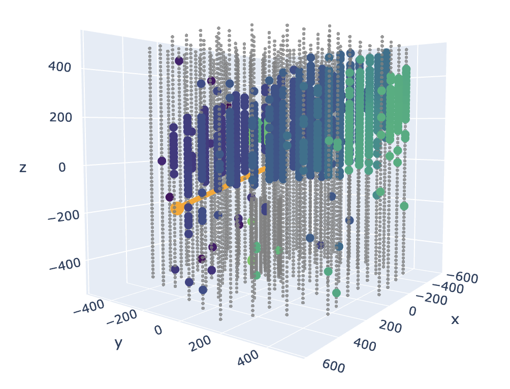
In the above plot, the gray dots represent sensors that did not detect any pulses in this event. Colored dots represent sensors that detected pulses, where darker blue ones are earlier pulses and lighter green are later in time. The orange line represents the neutrino’s direction. In this example, the orange line’s angle looks like a reasonable fit to the sensors that received pulses. This is a nicer-looking event; many events don’t show a clear track through the detector.
That’s it for exploratory data analysis. Next, we’ll look into how we can use principal component analysis to help reconstruct the neutrinos.
Principal Component Analysis
Principal component analysis (PCA) is a popular dimensionality reduction algorithm that works by identifying dimensions (for example, a plane) that lie closest to the data and then projecting the data onto it. In our case, we won’t be needing to project our data; we only need to find the best projection that preserves the maximum variance in the data, which will represent the neutrino’s direction.
PCA will find the axis that accounts for the largest amount of variance in the dataset, and it can also identify a second axis (orthogonal to the first one) that accounts for the largest amount of the remaining variance. It can also find a third axis (orthogonal to both of the previous axes), a fourth one, a fifth one, and so on, up to the number of dimensions in the dataset.
Before we perform PCA, let’s process our data by reading in a batch of data, only keeping higher-quality pulses (auxiliary=False), and dropping any repeated sensor pulses (for simplicity). We’ll also merge the data with our sensor geometry information.
Here’s the code (takes about 4 seconds to run):
# Read in parquet data for a single batch, and reset the index
batch_7 = pd.read_parquet('/Volumes/public/Python/icecube/train/batch_7.parquet')
batch_7 = batch_7.reset_index()

# Only keep higher-quality data
batch_7 = batch_7[batch_7['auxiliary'] == False]

# Ignore the charge columns since we won't be using them, and drop duplicates
batch_7 = batch_7[['event_id', 'sensor_id', 'time']]
batch_7 = batch_7.drop_duplicates(subset=['event_id', 'sensor_id'], keep='first')

# Read in sensor_geometry data, and merge with parquet data
sensor_geometry = pd.read_csv('/Volumes/public/Python/icecube/sensor_geometry.csv', low_memory=False)
batch_geo = pd.merge(batch_7, sensor_geometry, on='sensor_id', how='inner')
display(batch_geo.sample(5))
print(batch_geo.shape)
event_id	sensor_id	time	x	       y	      z
21788731	4848	    11586	41.60	   35.49	  -424.23
21980555	1290	    11135	-492.43	   -230.16	  -13.02
20913545	4093	    11275	-268.90	   354.24	  280.27
19707634	3729	    14347	-66.70	   276.92	  344.64
20113992	83	        9887	-132.80	   -501.45	  108.60

(4133016, 6)
The output shows that we have one detected pulse per row, with the time, sensor_id, and its geographical location (x, y, z) provided.
Let’s perform PCA by going through one event at a time, using scikit-learn’s PCA to fit to each event’s (x, y, z, t) data. We’ll be fitting to both unscaled and scaled data, to see if that affects the results. Also, we’ll make sure that the fitted PCA vector is pointing in the right direction.
This takes about 30 minutes to run:
from sklearn.preprocessing import StandardScaler
from sklearn.decomposition import PCA

# Define a DataFrame to hold the results
results = pd.DataFrame(columns=['event_id', 'pca_x', 'pca_y', 'pca_z', 'pca_var',
                                            'pca_s_x', 'pca_s_y', 'pca_s_z', 'pca_s_var',
])
results['event_id'] = results['event_id'].astype(int)

# Go through each unique event
for event_id in batch_geo['event_id'].unique():

    # Define the training data
    train = batch_geo[batch_geo['event_id'] == event_id][['x', 'y', 'z', 'time']].to_numpy()

    # Define the scaler, and scale the training data
    scaler = StandardScaler()
    scaled_train = scaler.fit_transform(train)

    # Fit PCA to both scaled and unscaled training data
    pca = PCA(n_components=1, svd_solver='full').fit(train)
    scaled_pca = PCA(n_components=1, svd_solver='full').fit(scaled_train)

    # If x and y are equal to 0, make x a small number so that the azimuth and zenith angles aren't undefined
    if (pca.components_[0][0] == 0) and (pca.components_[0][1] == 0):
        pca.components_[0][0] = 1e-06
    if (scaled_pca.components_[0][0] == 0) and (scaled_pca.components_[0][1] == 0):
        scaled_pca.components_[0][0] = 1e-06

    # Flip the direction of the PCA vectors if time is positive
    if pca.components_[0][3] > 0:
        pca.components_[0] = - pca.components_[0]
    if scaled_pca.components_[0][3] > 0:
        scaled_pca.components_[0] = - scaled_pca.components_[0]

    # Save all of this information to a DataFrame
    results.loc[len(results.index)] = [event_id, pca.components_[0][0], pca.components_[0][1], pca.components_[0][2], pca.explained_variance_ratio_[0],
                                                 scaled_pca.components_[0][0], scaled_pca.components_[0][1], scaled_pca.components_[0][2], scaled_pca.explained_variance_ratio_[0],
    ]

display(results.head(5))
print(results.shape)
	event_id	pca_x	    pca_y	        pca_z	    pca_var	    pca_s_x	    pca_s_y	    pca_s_z	    pca_s_var
0	19526675.0	-0.041279	-1.086727e-01	0.256477	0.991469	-0.465921	-0.502842	0.515349	0.906307
1	19539828.0	0.053141	3.337328e-02	0.180456	0.977748	0.512133	0.481357	0.536761	0.824943
2	19545811.0	-0.000000	3.330669e-16	0.185920	0.997839	-0.000001	0.000000	0.707107	0.984459
3	19548451.0	0.182637	-5.151474e-02	0.106419	0.941337	0.580503	-0.553344	0.120713	0.650493
4	19552579.0	0.187720	-7.183004e-02	0.189596	0.994454	0.501781	-0.501781	0.500839	0.978909

(200000, 9)
Looks great. Now we have a DataFrame with 200,000 rows (one per event), with each row giving us the neutrino’s xyz orientation and the amount of variance captured. We have this information for both unscaled and scaled (contains _s in the column labels) data. We also notice that the unscaled data has higher captured variance than the scaled data.
The next step is to convert our results from cartesian (xyz) to spherical (azimuth, zenith) coordinates, since the latter is the form that our ground truth labels use. We’ll also make sure that our angles are always positive.
Make the conversions:
# Convert from cartesian to spherical coordinates to get the direction of the event — designed to work on DataFrame columns
def cart_to_spherical(df_x, df_y, df_z):
    x2_and_y2 = (df_x ** 2) + (df_y ** 2)
    zenith = np.arccos(df_z / np.sqrt(x2_and_y2 + (df_z ** 2)))
    azimuth = np.sign(df_y) * np.arccos(df_x / np.sqrt(x2_and_y2))
    return azimuth, zenith

# Make conversions
results['pca_azi'], results['pca_zen'] = cart_to_spherical(results['pca_x'], results['pca_y'], results['pca_z'])
results['pca_s_azi'], results['pca_s_zen'] = cart_to_spherical(results['pca_s_x'], results['pca_s_y'], results['pca_s_z'])

# Convert from (-pi, +pi) to (0, 2pi) — this is for single values, not DataFrame columns
def angle_to_2pi(angle):
    angle_2pi = angle % (2 * np.pi)
    if angle_2pi < 0:
        angle_2pi += 2 * np.pi
    return angle_2pi

# Fix angles
results['pca_azi'] = results['pca_azi'].apply(angle_to_2pi)
results['pca_s_azi'] = results['pca_s_azi'].apply(angle_to_2pi)

display(results.head(5))
print(results.shape)
event_id	pca_x	    pca_y	        pca_z	    pca_var	    pca_s_x	    pca_s_y	    pca_s_z	    pca_s_var	pca_azi	    pca_zen	    pca_s_azi	pca_s_zen
19526675.0	-0.041279	-1.086727e-01	0.256477	0.991469	-0.465921	-0.502842	0.515349	0.906307	4.349375	0.425555	3.965084	0.926164
19539828.0	0.053141	3.337328e-02	0.180456	0.977748	0.512133	0.481357	0.536761	0.824943	0.560759	0.334660	0.754430	0.918582
19545811.0	-0.000000	3.330669e-16	0.185920	0.997839	-0.000001	0.000000	0.707107	0.984459	1.570796	0.000000	0.000000	0.000001
19548451.0	0.182637	-5.151474e-02	0.106419	0.941337	0.580503	-0.553344	0.120713	0.650493	6.008266	1.059700    5.521735	1.421400
19552579.0	0.187720	-7.183004e-02	0.189596	0.994454	0.501781	-0.501781	0.500839	0.978909	5.917729	0.814570	5.497787	0.956203

(200000, 13)
Now our DataFrame has four additional columns: azimuth and zenith, for both unscaled and scaled data.
To compare our results with the ground truth labels, let’s add the labels to our DataFrame:
# Get ground truth labels
train_meta = pd.read_parquet('/Volumes/public/Python/icecube/train_meta.parquet')
train_meta = train_meta[['event_id', 'azimuth', 'zenith']]

# Add ground truth labels to the DataFrame
results['event_id'] = results['event_id'].astype(int)
results = pd.merge(results, train_meta, on='event_id', how='left')
We’ll also define a function to calculate the angular error between two angles:
def angular_dist(az_true, zen_true, az_pred, zen_pred):

    if not (np.all(np.isfinite(az_true)) and
            np.all(np.isfinite(zen_true)) and
            np.all(np.isfinite(az_pred)) and
            np.all(np.isfinite(zen_pred))):
        raise ValueError("All arguments must be finite")

    # Pre-compute all sine and cosine values
    sa1 = np.sin(az_true)
    ca1 = np.cos(az_true)
    sz1 = np.sin(zen_true)
    cz1 = np.cos(zen_true)

    sa2 = np.sin(az_pred)
    ca2 = np.cos(az_pred)
    sz2 = np.sin(zen_pred)
    cz2 = np.cos(zen_pred)

    # Scalar product of the two cartesian vectors (x = sz*ca, y = sz*sa, z = cz)
    scalar_prod = sz1*sz2*(ca1*ca2 + sa1*sa2) + (cz1*cz2)

    # Scalar product of two unit vectors is always between -1 and 1, this is against nummerical instability
    scalar_prod =  np.clip(scalar_prod, -1, 1)

    # Convert back to an angle (in radian)
    return np.abs(np.arccos(scalar_prod))
Calculate the mean angular error between our results and ground truth labels, and plot them as histograms:
# Calculate the angular error
pca_error = angular_dist(results['azimuth'],
                         results['zenith'],
                         results['pca_azi'],
                         results['pca_zen'])
pca_s_error = angular_dist(results['azimuth'],
                           results['zenith'],
                           results['pca_s_azi'],
                           results['pca_s_zen'])
print(f'PCA: {np.average(pca_error):.2f} rad')
print(f'PCA-scaled: {np.average(pca_s_error):.2f} rad')
results['pca_error'] = pca_error

# Make histogram plots
fig, (ax1, ax2) = plt.subplots(1, 2, figsize=(13, 5))
ax1.hist(pca_error, bins=20, label='PCA Model', fc=(1, 0.5, 0.2, 0.5), range=(0, np.pi))
ax1.set_title('Angular Error')
ax1.set_xlabel('Ground Truth Difference [rad]')
ax1.set_ylabel('Count')
ax1.legend()
ax2.hist(pca_s_error, bins=20, label='Scaled PCA Model', fc=(0, 0.5, 1, 0.5), range=(0, np.pi))
ax2.set_title('Angular Error')
ax2.set_xlabel('Ground Truth Difference [rad]')
ax2.set_ylabel('Count')
ax2.legend()
plt.show()
PCA: 1.21 rad
PCA-scaled: 1.27 rad
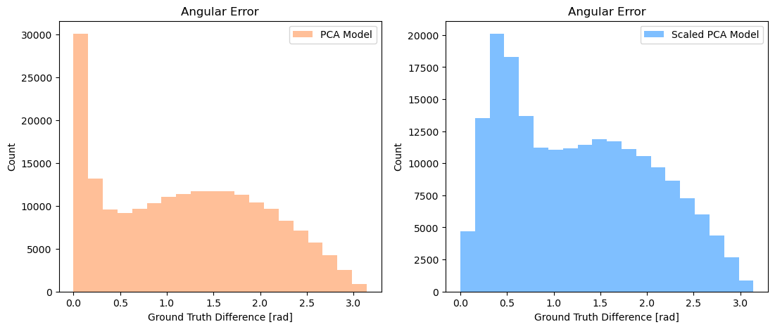
PCA on unscaled data performs better than using it on scaled data. We already saw earlier that unscaled data resulted in a larger amount of captured variance. Looking at the histograms, unscaled PCA has more events with lowest error (in the leftmost histogram bin) compared to scaled PCA. Both PCA histograms show a distribution centered around π/2, which is what we would expect from random guessing of the neutrino’s direction. It appears that the neutrino events in our dataset are either (1) straightforward to determine the correct angle, or (2) difficult to determine such that PCA can’t do better than random guessing.
Now that we know that PCA can yield results of ~1.21 radians for the mean angular error, let’s see how well we can do using neural networks in the next section.
Recurrent Neural Networks
In this section, I’ll discuss my work on training recurrent neural networks (RNNs) and their flavors such as gated recurrent units (GRUs) and long short-term memory (LSTMs) to reconstruct a neutrino event. RNNs are a class of neural networks that analyze time series data, and are commonly used for forecasting and natural language processing.
To use these models, I’ll be treating the data as a time series or sequence. Each neutrino event will be defined by a sequence composed of sensor IDs listed in the order in which pulses are detected. Since events vary in the number of sensors triggered, different sequences can have different lengths. I will define a maximum sequence length so that any sequences longer than that will be truncated, and I will define a padding value (0) to pad sequences shorter than the maximum sequence length.
Here’s a Python script that pre-processes all of the IceCube data files, with optional command line arguments to specify the train-validation splitting fraction and maximum sequence length. It takes about 1 minute per parquet file or about 8 hours for the entire dataset:
# -----------------------------------------------------------------------------
# Imports

import argparse
import glob
import pandas as pd
import numpy as np
import csv


# -----------------------------------------------------------------------------
# Process parquet files

def process_data(input_file, split_name):

    # Read the input file, and reset the index
    batch = pd.read_parquet(input_file)
    batch = batch.reset_index()

    # Only keep higher-quality data
    batch = batch[batch['auxiliary'] == False]

    # Ignore the charge columns since we won't be using them, and re-order sensor_id in order of time
    batch = batch[['event_id', 'sensor_id', 'time']]
    batch = batch.sort_values(by=['event_id', 'time'], axis=0, ascending=True)

    # Add sensor_id by 1: 0-5159 --> 1-5160 because the 0 token is reserved for padding
    batch['sensor_id'] = batch['sensor_id'] + 1

    # Create a nested list of all events [ [event #1's sensors in order], [event #2's sensors in order], ...] and corresponding IDs
    g = batch.groupby('event_id')
    events = g['sensor_id'].apply(list).tolist()
    event_ids = list(g.groups.keys())

    # Truncate events longer than the maximum sequence length
    events = [e[:args.sequencelen] for e in events]

    # Pad events with 0, if shorter than the maximum sequence length
    events = [e + [0] * (args.sequencelen - len(e)) for e in events]

    # Get target values (labels)
    labels = meta.reindex(event_ids).values.tolist()

    # Combine the events and labels into a single list
    events_labels = [e + l for e, l in zip(events, labels)]

    # Save as CSV file
    with open(args.outputdir+split_name+'_'+input_file.split('/')[-1].split('.')[0][6:]+'.csv', 'w') as f:
        write = csv.writer(f)
        write.writerows(events_labels)


# -----------------------------------------------------------------------------

if __name__ == "__main__":

    # Define command line arguments
    parser = argparse.ArgumentParser(description='IceCube data preprocessing')
    parser.add_argument('-metafile', type=str, default='/Volumes/public/Python/icecube/train_meta.parquet', help='metadata filepath')
    parser.add_argument('-parquetdir', type=str, default='/Volumes/public/Python/icecube/train/', help='filepath for the directory containing parquet files')
    parser.add_argument('-trainfrac', type=float, default=0.9, help='fraction of the dataset to be used for the training set')
    parser.add_argument('-sequencelen', type=int, default=300, help='max length of each example in the dataset')
    parser.add_argument('-outputdir', type=str, default='/Volumes/public/Python/icecube/train_2023-02-27/', help='filepath for the output directory')

    # Parse arguments
    args = parser.parse_args()

    # Read the metadata file
    print(f'Reading metadata file...')
    meta = pd.read_parquet(args.metafile)
    meta = meta[['event_id', 'azimuth', 'zenith']]
    meta = meta.set_index('event_id')

    # Grab all of the parquet files, shuffle, and split into training/validation sets
    parquets = glob.glob(args.parquetdir + '*.parquet')
    print(f'Found {len(parquets)} parquet files')
    parquets = np.random.permutation(parquets)
    train_parquets = parquets[:int(len(parquets) * args.trainfrac)]
    valid_parquets = parquets[int(len(parquets) * args.trainfrac):]
    print(f'Split into {len(train_parquets)} training parquets and {len(valid_parquets)} validation parquets')

    # For each parquet file, pre-process the dataset and save to file
    for parquet in train_parquets:
        print(f'Processing train {parquet}')
        process_data(parquet, split_name='train')
    for parquet in valid_parquets:
        print(f'Processing valid {parquet}')
        process_data(parquet, split_name='valid')
After running this script, we’ll have one pre-processed CSV file per input parquet file. We’ll use these CSV files as inputs to train our neural networks.
I have publicly uploaded my pre-processed CSV datasets to Kaggle: IceCube Training Data and IceCube Validation Data. If you prefer using SQL, I have also uploaded them as a SQLite database: IceCube SQL Data.
Just prior to training, data are read from the CSV files into memory, truncated (if desired), and converted to PyTorch tensors. A Dataset class is defined to read in a single row from the tensor at a time, and a DataLoader is defined to load a batch of rows.
For example, this is how we define the validation set:
class IceCubeDataset(Dataset):
    def __init__(self, data, targ):
        self.data = data
        self.targ = targ

    def __len__(self):
        return len(self.targ)

    def __getitem__(self, idx):
        return self.data[idx], self.targ[idx]

valid_df = pd.read_csv(valid_filepath, names=range(302))
valid_data = torch.tensor(valid_df.iloc[:, :args.trunc].values, dtype=torch.long)
valid_targ = torch.tensor(valid_df.iloc[:, -2:].values, dtype=torch.float32)
valid_dataset = IceCubeDataset(valid_data, valid_targ)
valid_dl = DataLoader(valid_dataset, batch_size=args.bs, shuffle=False, num_workers=args.workers, pin_memory=pinning_mem)
I ended up assigning only a single CSV file as my validation set since more were unnecessary. All remaining 659 CSV files were assigned to the training set. In every epoch, I would iterate through the entire CSV set once, and then move on to the next CSV file in the next epoch. In total, this meant that the model would train for 659 epochs without ever seeing the same neutrino event more than once, therefore eliminating the possibility of overfitting.
Regarding the type of sequential model, I experimented with vanilla RNNs, GRUs, and LSTMs. The latter two equally outperformed the former, so I proceeded with the GRU only for all subsequent experiments.
Here’s the model class for the GRU network:
class GRUModel(nn.Module):
    def __init__(self, vocab_size, emb_dim, hidden_dim, n_layers, fc1_dim, output_size):
        super().__init__()
        self.vocab_size = vocab_size
        self.emb_dim = emb_dim
        self.hidden_dim = hidden_dim
        self.n_layers = n_layers
        self.fc1_dim = fc1_dim
        self.output_size = output_size

        self.embedding = nn.Embedding(num_embeddings=self.vocab_size, embedding_dim=self.emb_dim, padding_idx=0)

        self.gru = nn.GRU(input_size=self.emb_dim, hidden_size=self.hidden_dim, num_layers=self.n_layers,
                          bias=True, batch_first=True, bidirectional=False)
        for name, param in self.gru.named_parameters():
            if 'bias' in name:
                nn.init.constant_(param, 0.0)
            elif 'weight_ih' in name:
                nn.init.xavier_uniform_(param, nn.init.calculate_gain('tanh'))
            elif 'weight_hh' in name:
                nn.init.orthogonal_(param, nn.init.calculate_gain('tanh'))

        self.fc1 = nn.Linear(self.hidden_dim, self.fc1_dim)
        for name, param in self.fc1.named_parameters():
            if 'bias' in name:
                nn.init.constant_(param, 0.0)
            elif 'weight' in name:
                nn.init.xavier_uniform_(param, gain=nn.init.calculate_gain('relu'))

        self.relu = nn.ReLU()

        self.fc2 = nn.Linear(self.fc1_dim, self.output_size)
        for name, param in self.fc2.named_parameters():
            if 'bias' in name:
                nn.init.constant_(param, 0.0)
            elif 'weight' in name:
                nn.init.xavier_uniform_(param, gain=1)

    def forward(self, x):
        seq_lengths = torch.count_nonzero(x, dim=1)
        gru_output, _ = self.gru(self.embedding(x))
        output_last = torch.stack([gru_output[i, l - 1, :] for i, l in enumerate(seq_lengths)], dim=0)
        final_output = self.fc2(self.relu(self.fc1(output_last)))

        return final_output
The first layer is an embedding layer; each sequence element (which is an IceCube sensor ID) is converted to a vector of numbers via a lookup table. This embedding vector is a quantitative representation of each sensor ID in the neural network. The second layer is the GRU (see torch.nn.GRU). The third layer is a fully connected layer with a ReLU activation, and the fourth layer is the output layer.
Training is done using the PyTorch framework, experiment tracking is performed using Neptune.ai, and hardware was either my local machine (CPU) or Lambda Labs (GPU).
Here are some of the hyperparameters corresponding to my best models:
- L1Loss for the loss function
- AdamW for the optimizer
- Cosine annealing for the scheduler
- Embedding dimension of 10
- GRU had 50 hidden units and 1 layer
- Fully connected layer of 30 units
- Batch size of 1024
- Learning rate of 0.006
These plots show the loss vs. epoch (top) and the mean angular error vs. epoch (bottom), for both training and validation sets:
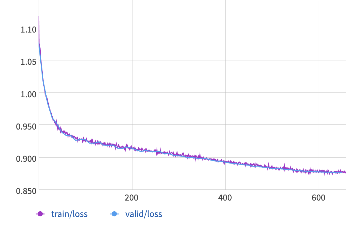
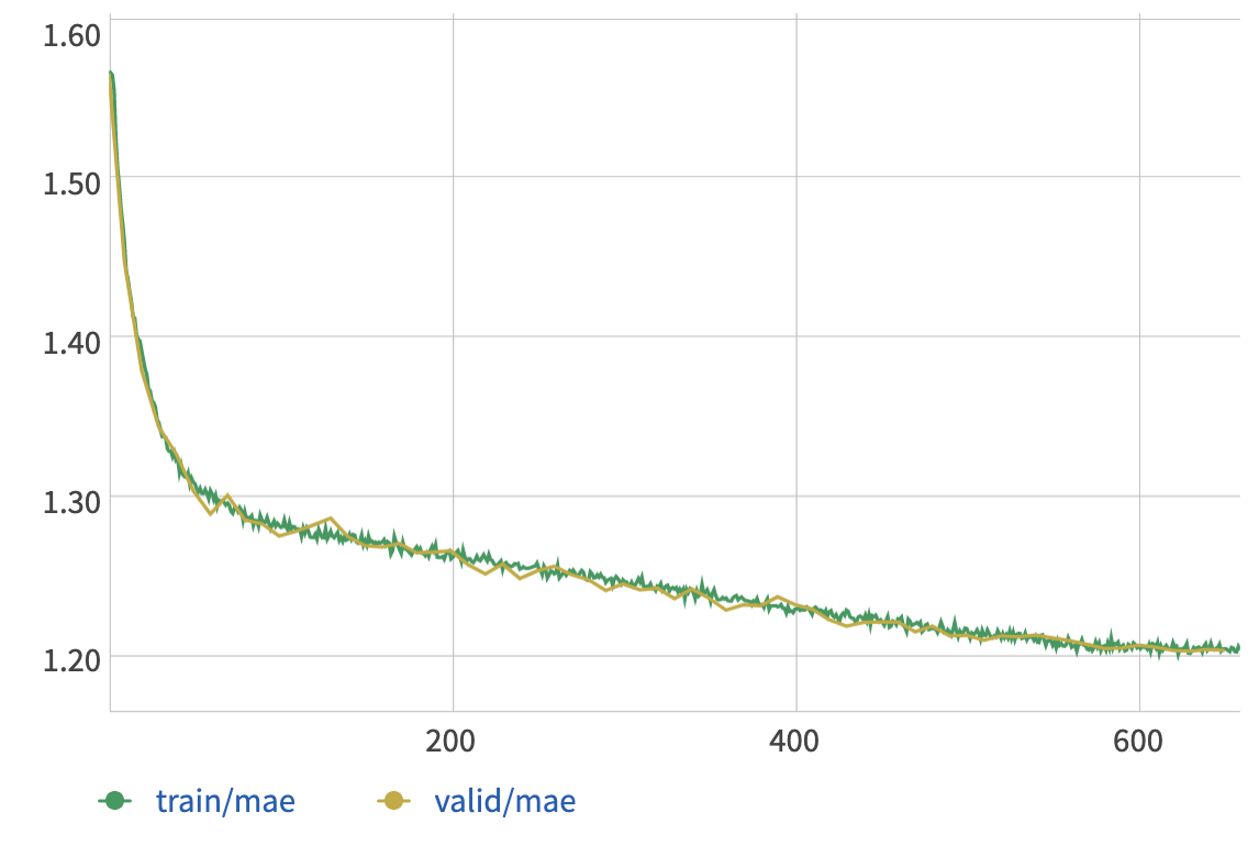
The GRU model converges to about 1.20 radians for the mean angular error, which is only slightly better than the results from PCA.
Overall, I would say that the biggest gains in model improvement were obtained by (1) upgrading from a vanilla RNN to a GRU or LSTM, and (2) training on the entire dataset. The remaining hyperparameters only had minor effects.