Getting Started With PyTorch For Computer Vision

October 9, 2022 2102 words 10 minutes

Contents

Introduction

In this blog post, I’m going to walk through my process implementing transfer learning in a computer vision classification problem using the PyTorch framework. I’ll briefly introduce the dataset used here, then cover the training (sweeping hyperparameters and fine-tuning a model) and inference steps. This post is designed for people who are new to PyTorch or just getting started with it.

Interested in applying PyTorch to a tabular dataset (i.e., structured data like a spreadsheet) instead? Check out this post: Getting Started With PyTorch Using Tabular Data.

Dataset

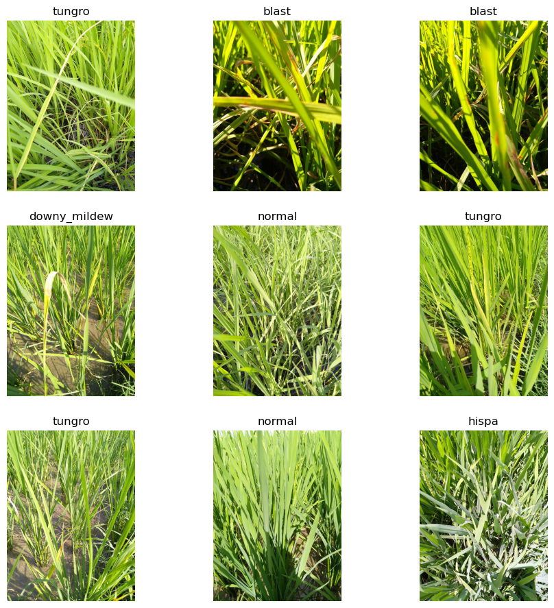
The first step is to explore the image dataset. I’ll be using a dataset of rice crop images from Kaggle’s Paddy Disease Classification competition, which includes about 10,000 training examples of crops with 9 disease classes and 1 normal (undiseased) class.

Write a function to plot some random images:

def plot_random_images(img_dir):
    img_dataset = datasets.ImageFolder(img_dir)
    class_names = img_dataset.classes

    fig = plt.figure(figsize=(11, 11))
    rows, cols = 3, 3

    for i in range(1, rows * cols + 1):
        random_idx = torch.randint(0, len(img_dataset), size=[1]).item()
        img, label = img_dataset[random_idx]
        fig.add_subplot(rows, cols, i)
        plt.imshow(img)
        plt.title(class_names[label])
        plt.axis(False)
    plt.show()

This function takes in a directory path of images, loads them according to PyTorch’s ImageFolder class (where every image is in a subfolder named after the image’s class), and plots a 3x3 grid of random images alongside their class label.

Plot random images:

data.plot_random_images('train_images/')

Write a function to check image dimensions:

def check_img_dim(data_dir, file_ext='.jpg'):
    train_sizes = pd.Series(dtype=str)

    # Go through the base folder
    with os.scandir(data_dir) as base_entries:
        for base_entry in base_entries:
            if base_entry.is_dir():

                # Go through each subfolder
                with os.scandir(data_dir + base_entry.name) as entries:
                    for entry in entries:
                        if entry.name.endswith(file_ext):

                            # Get image dimensions (im_width, im_height = im.size)
                            im = Image.open(data_dir + base_entry.name + '/' + entry.name)
                            train_sizes = pd.concat([train_sizes, pd.Series(str(im.size))], axis=0)

    print(train_sizes.value_counts())

This function scans the image directory to check the dimensions of each image, and provides a printout of the frequency of each dimension.

Check image dimensions:

data.check_img_dim('train_images/')

(480, 640)    10403
(640, 480)        4
dtype: int64

Almost all images are 480x640, with just 4 images that are 640x480.

Training

Before we get started with training, I want to mention that I have everything set up in Python scripts, not a Jupyter notebook environment. My functions reside in a separate folder called utils, which contain scripts organized by function type (e.g., models.py contains functions related to defining PyTorch models). If you decide to do something similar, I suggest creating a path configuration file so that your functions can be imported into Python.

I used both GPU and CPU for training. For the former, I used a cloud GPU service called Jarvislabs.ai for its ease of setup and affordable prices, and for the latter, I used my local CPU which is a Mac machine with 8 cores and 64 GB memory. If you haven’t used cloud GPU providers before, I would say that the main downside is the setup required to install packages, download datasets, etc. every time you start up a new instance. However, Jarvislabs.ai has a handy option to “pause” an instance. I recommend writing your code in a device-agnostic manner so that it works on either the GPU or the CPU, as you’ll see in my code examples below.

Since transfer learning will be based on Torchvision’s models and pre-trained weights, I am using their new API which requires Torchvision version 0.13 or above. Check your version, and if needed, install a different version using the install command builder for your system (select nightly build) or install from the previous versions page with Torchvision 0.13+.

Check PyTorch and Torchvision versions:

print('[INFO] PyTorch v.', torch.__version__, '| Torchvision v.', torchvision.__version__)

Set up device-agnostic code where device will be assigned either cpu or gpu (and print the model of the NVIDIA GPU):

device = 'cuda' if torch.cuda.is_available() else 'cpu'
print(f'[INFO] Using {device}.')
if device == 'cuda':
    print(f'[INFO] {torch.cuda.get_device_name(device)}')

Define relevant directories:

data_dir = 'datasets/'
model_dir = 'models/'
runs_dir = 'runs/'

These variables specify the directory paths of where the training dataset is located, where models should be saved, and where run results should be saved.

Set up training hyperparameters:

params = {
    'num_epochs': [5],
    'batch_size': [32],
    'learning_rate': [0.01],
    'model': [models.create_convnext_tiny]
}
param_grid = ParameterGrid(params)

The params dictionary specifies the value (or a list of values to sweep through) for each hyperparameter. For the model parameter, models.create_convnext_tiny refers to the name of a function that will create a ConvNeXt Tiny model. Lastly, ParameterGrid is imported from sklearn.model_selection and will create an iterable to go through all permutations of the parameter grid.

I recommend starting off with a small number of epochs, like 5 or so. This allows a run to finish quickly if it isn’t yielding useful results. If it is giving good results, you can easily continue where it left off by loading the saved model as your next run’s starting point.

Is your model taking too long to train? Try increasing the batch size, which will reduce the number of total batches but will also reduce the number of times that gradient descent is performed.

Set up a hyperparameter loop:

# Define an experiment ID and whether to continue from a previously saved model
exp_id = 24
continue_model = '../23.pth'

results = []

for grid in param_grid:

    # Instantiate a model and start from previous model
    model, weights = grid['model'](out_features=10, device=device)
    if continue_model != '':
        model.load_state_dict(torch.load(f=continue_model, map_location=torch.device(device)))
        model.to(device)
        print(f'[INFO] Starting from {continue_model}')

    # Create data transforms
    data_transform = weights.transforms()

    # Create train/validation dataloaders
    train_dl, valid_dl, class_names = data.load_images_and_split(
        img_dir=data_dir+'train_images/', 
        valid_fraction=0.25, 
        transform=data_transform, 
        batch_size=grid['batch_size'], 
        num_workers=0
    )

    # Select a loss function and an optimizer
    loss_fn = torch.nn.CrossEntropyLoss()
    optimizer = torch.optim.SGD(model.parameters(), lr=grid['learning_rate'])

    # Train the model
    print(f'------------- exp_id = {exp_id} ({datetime.now().strftime("%Y-%m-%d %H:%M:%S")}) -------------')
    writer = training.create_writer(
        runs_dir=runs_dir,
        model_name=grid['model'].__name__, 
        experiment_name=str(exp_id), 
        lr=str(grid['learning_rate']),
        bs=str(grid['batch_size'])
    )
    model_results = training.train_acc(
        model=model,
        train_dataloader=train_dl,
        test_dataloader=valid_dl,
        loss_fn=loss_fn,
        optimizer=optimizer,
        epochs=grid['num_epochs'],
        device=device,
        writer=writer
    )

    # Save the model's results to a list of dicts
    model_results.update({'exp_id': exp_id})
    model_results.update(grid)
    results.append(model_results)

    # Save the model to file
    training.save_torch_model(
        model=model,
        target_dir=model_dir,
        model_name=f'{exp_id}.pth'
    )

    exp_id += 1

I’ve included some comments above to explain what the code is doing, but I’ll describe some of the steps in more detail below.

The first step is the creation of a pre-trained model, which includes instantiation, freezing of layers, and adjusting the output layer for the number of desired output classes (10 in my case). To view the architecture of a given model, you can simply print(model) or use torchinfo’s summary command (Github) to print a table of its layers.

Example of a function to create a model:

def create_convnext_tiny(out_features, device):

    weights = torchvision.models.ConvNeXt_Tiny_Weights.DEFAULT
    model = torchvision.models.convnext_tiny(weights=weights).to(device)

    for param in model.features.parameters():
        param.requires_grad = False

    model.classifier = nn.Sequential(
        torchvision.models.convnext.LayerNorm2d((768,), eps=1e-06, elementwise_affine=True),
        nn.Flatten(start_dim=1, end_dim=-1),
        nn.Linear(in_features=768, out_features=out_features, bias=True)
    ).to(device)
    
    model.name = 'ConvNeXt Tiny'
    print(f'[INFO] Created new {model.name} model.')

    return model, weights

The next step is to apply the same transforms used in the pre-trained model to the dataset.

View the transforms used in the pre-trained model:

weights.transforms()

ImageClassification(
    crop_size=[224]
    resize_size=[236]
    mean=[0.485, 0.456, 0.406]
    std=[0.229, 0.224, 0.225]
    interpolation=InterpolationMode.BILINEAR
)

Using these transforms, we can create a DataLoader (docs), which is what PyTorch uses to fetch data and serve in batches. I wrote a function to simultaneously define the DataLoader objects and split the data into training and validation sets.

Example of a function to create DataLoader:

def load_images_and_split(img_dir, valid_fraction, transform, batch_size=32, num_workers=0):

    # Use ImageFolder to read the dataset
    img_dataset = datasets.ImageFolder(img_dir, transform=transform)

    # Get class names
    class_names = img_dataset.classes

    # Split the dataset into training and validation sets
    valid_size = int(len(img_dataset) * valid_fraction)
    train_size = len(img_dataset) - valid_size
    train_data, valid_data = random_split(img_dataset, [train_size, valid_size])

    # Turn images into data loaders
    train_dataloader = DataLoader(
        train_data,
        batch_size=batch_size,
        shuffle=True,
        num_workers=num_workers,
        pin_memory=True,
    )
    valid_dataloader = DataLoader(
        valid_data,
        batch_size=batch_size,
        shuffle=True,
        num_workers=num_workers,
        pin_memory=True,
    )

    return train_dataloader, valid_dataloader, class_names

The length of each DataLoader is equal to the number of batches needed to go through all of the images. The output class_names above is a list of the classes for my particular dataset (e.g., ‘bacterial_panicle_blight’, ‘blast’, ‘brown_spot’, etc.).

Before training the model, I define the loss function (cross entropy), optimizer (stochastic gradient descent), and TensorBoard writer (see PyTorch docs) to track my runs (e.g., metrics like classification accuracy and validation loss) and plot them. The create_writer function specifies a logging directory where the runs will be stored.

The next step is actually training the model. I have a function train_acc that loops through each epoch, calling a training function train_step_acc and an evaluation function test_step_acc as well as recording metrics.

Examples of functions to perform training and evaluation:

def train_acc(model, train_dataloader, test_dataloader, optimizer, loss_fn, epochs, device, writer=None):

    # Loop through training and testing steps for a number of epochs
    for epoch in range(epochs):
        train_loss, train_acc = train_step_acc(model=model,
            dataloader=train_dataloader,
            loss_fn=loss_fn,
            optimizer=optimizer,
            device=device)
        test_loss, test_acc = test_step_acc(model=model,
            dataloader=test_dataloader,
            loss_fn=loss_fn,
            device=device)

        # Print out what's happening
        print(
            f'{datetime.now().strftime("%Y-%m-%d %H:%M:%S")} | EPOCH {epoch+1:3.0f} | '
            f'TRAIN loss: {train_loss:.4f} acc: {train_acc:.4f} | '
            f'TEST loss: {test_loss:.4f} acc: {test_acc:.4f}'
        )

        # Experiment tracking
        if writer:
            writer.add_scalars(main_tag='loss', tag_scalar_dict={'train': train_loss, 'test': test_loss}, global_step=epoch)
            writer.add_scalars(main_tag='accuracy', tag_scalar_dict={'train': train_acc, 'test': test_acc}, global_step=epoch)
            writer.add_graph(model=model, input_to_model=torch.randn(32, 3, 224, 224).to(device))
            writer.close()

        # Create a results dictionary at the last epoch
        if epoch + 1 == epochs:
            results = {
                "train_loss": train_loss,
                "train_acc": train_acc,
                "test_loss": test_loss,
                "test_acc": test_acc
            }

    # Return the results
    return results

def train_step_acc(model, dataloader, loss_fn, optimizer, device):

    model.train()

    train_loss, train_acc = 0, 0

    for batch, (X, y) in enumerate(dataloader):

        X, y = X.to(device), y.to(device)
        y_pred = model(X)

        loss = loss_fn(y_pred, y)
        train_loss += loss.item() 

        optimizer.zero_grad()
        loss.backward()
        optimizer.step()

        y_pred_class = torch.argmax(torch.softmax(y_pred, dim=1), dim=1)
        train_acc += (y_pred_class == y).sum().item()/len(y_pred)

    train_loss = train_loss / len(dataloader)
    train_acc = train_acc / len(dataloader)

    return train_loss, train_acc

def test_step_acc(model, dataloader, loss_fn, device):

    model.eval() 

    test_loss, test_acc = 0, 0

    with torch.inference_mode():
        for batch, (X, y) in enumerate(dataloader):
 
            X, y = X.to(device), y.to(device)

            test_pred_logits = model(X)

            loss = loss_fn(test_pred_logits, y)
            test_loss += loss.item()

            test_pred_labels = test_pred_logits.argmax(dim=1)
            test_acc += ((test_pred_labels == y).sum().item()/len(test_pred_labels))

    test_loss = test_loss / len(dataloader)
    test_acc = test_acc / len(dataloader)

    return test_loss, test_acc

The last step is to save the model’s parameters, which are stored in a dictionary called state_dict and can be saved using torch.save(obj=model.state_dict(), f=model_save_path).

And that’s it — all of the above steps should get you started on fine-tuning a pre-trained model as well as sweeping hyperparameter values.

Inference

Once you have some saved models that you’re satified with, you can perform inference by generating predictions on a test set.

Recall the class_names we obtained earlier? The first step is to create a mapping dictionary of those classes.

Define a mapping dictionary for the classes:

class_names = [
    'bacterial_leaf_blight',
    'bacterial_leaf_streak',
    'bacterial_panicle_blight',
    'blast',
    'brown_spot',
    'dead_heart',
    'downy_mildew',
    'hispa',
    'normal',
    'tungro'
]
mapping_dict = dict(enumerate(class_names))

Define the directory paths where the models are located and instantiate a model:

models_list = [
    '../24.pth',
    '../25.pth'
]
model, _ = models.create_convnext_tiny(out_features=10, device=device)

Note that I’m assuming your models all stem from the same pre-trained model. If that’s not the case, you’ll need to run a separate script for each model type or define them separately.

Define a generic transform for the test set:

image_transform = transforms.Compose([
    transforms.Resize((224, 224)),
    transforms.ToTensor(),
    transforms.Normalize(mean=[0.485, 0.456, 0.406], std=[0.229, 0.224, 0.225])
])

Create a DataLoader for the test set:

test_dir = '../test_images/'
test_data = datasets.ImageFolder(test_dir, transform=image_transform)
test_dl = DataLoader(
    test_data,
    batch_size=32,
    shuffle=False,
    num_workers=0,
    pin_memory=True,
)

Note that shuffle=False, so we know which image names correspond to which predictions. In order to use ImageFolder for the test data, I moved the test images into a subfolder called no_label to follow the ImageFolder convention.

Get the image names associated with the test set:

fnames_classes = test_dl.sampler.data_source.imgs
fnames = [f[0].replace(test_dir + 'no_label/', '') for f in fnames_classes]

Great. Now I’m going to loop through all of the models in models_list, and for each of them, I’m going to generate predictions, create a submissions CSV, and submit to Kaggle via their API.

Loop through all models:

for m in models_list:

    # Load saved model
    model.load_state_dict(torch.load(f=m, map_location=torch.device(device)))
    model.to(device)

    # Generate predictions
    test_pred_class = analysis.eval_model(model, test_dl, device)

    # Create a DataFrame with predictions
    submission = pd.DataFrame(columns=['image_id', 'label'])
    submission['image_id'] = fnames
    submission['label'] = test_pred_class
    submission['label'] = submission['label'].map(mapping_dict)

    # Save to CSV
    submission.to_csv(m[:-4] + '-submission.csv', index=False)

    # Submit to Kaggle
    os.system(f'kaggle competitions submit -f {m[:-4]}-submission.csv -m "submission" -q "paddy-disease-classification"')

The actual evaluation was performed in a function called eval_model:

def eval_model(model, test_data_loader, device):
    test_pred_class = []
    model.eval()
    with torch.inference_mode():
        for i, (X, _) in enumerate(test_data_loader, 0):
            X = X.to(device)
            test_pred = model(X)
            test_pred_class.append(torch.argmax(torch.softmax(test_pred, dim=1), dim=1))
    return torch.cat(test_pred_class)

And that’s it! We have successfully generated predictions based on our best models.

Resources

Learn PyTorch for Deep Learning: Zero to Mastery for in-depth PyTorch tutorials
PyTorch Image Models (timm)
Which image models are best? notebook for performance plots of computer vision models
Paddy Disease Classification notebooks: 1 2 3 4