Getting Started With PyTorch Using Tabular Data

Introduction
This tutorial introduces the PyTorch framework by applying it to a tabular dataset (i.e., structured data like a spreadsheet). It’s ideal for someone who is completely new to PyTorch, but has experience using other machine learning libaries. The goal is to help you get PyTorch up and running using a simple dataset and model.
If you’re not familiar with PyTorch, it’s an open source machine learning framework designed for deep learning applications including computer vision and natural language processing. It was originally developed by Meta AI, and is now part of The Linux Foundation.
You don’t need a GPU to follow along this tutorial; running PyTorch on your CPU will be adequate for our computational needs. If it’s not already installed, your first step should be to install PyTorch on your local machine. Follow the instructions on PyTorch’s Getting Started page by selecting a build and other options to generate a run command.
The next step is to open up Python (either a notebook or script environment) and import modules:
import torch
from torch import nn

from sklearn.model_selection import train_test_split

import numpy as np
import pandas as pd

import matplotlib as mpl
import matplotlib.pyplot as plt

from kaggle import api

from pathlib import Path

# Settings for matplotlib
%matplotlib inline
mpl.rc('axes', labelsize=14)
mpl.rc('xtick', labelsize=12)
mpl.rc('ytick', labelsize=12)

# Specify float format for pandas tables
pd.options.display.float_format = '{:.3f}'.format
I’ve installed and imported kaggle because I use their API to automatically submit to competitions (see Inference & Submission section). You can skip this if you don’t want to use their API.
We’re going to be using the Titanic dataset (Kaggle competition page) to create a model to predict the passengers that survive the shipwreck. This is a classification problem — for each passenger, I will predict 0 (deceased) or 1 (survived). I recommend creating a Kaggle account so that you can download the datasets and follow along the tutorial.
Feature Engineering
Now that everything is set up, I’m going to perform some feature engineering and data cleaning before I get to the fun training part using PyTorch.
Read in the training and test sets from CSV files:
df = pd.read_csv('../titanic/train.csv')
test_df = pd.read_csv('../titanic/test.csv')

df.info()
<class 'pandas.core.frame.DataFrame'>
RangeIndex: 891 entries, 0 to 890
Data columns (total 12 columns):
 #   Column       Non-Null Count  Dtype
---  ------       --------------  -----
 0   PassengerId  891 non-null    int64
 1   Survived     891 non-null    int64
 2   Pclass       891 non-null    int64
 3   Name         891 non-null    object
 4   Sex          891 non-null    object
 5   Age          714 non-null    float64
 6   SibSp        891 non-null    int64
 7   Parch        891 non-null    int64
 8   Ticket       891 non-null    object
 9   Fare         891 non-null    float64
 10  Cabin        204 non-null    object
 11  Embarked     889 non-null    object
dtypes: float64(2), int64(5), object(5)
memory usage: 83.7+ KB
None
Note that Survived is the column that I am trying to predict. Pclass is the ticket class (e.g., 1 for 1st class), SibSp is the number of siblings/spouses aboard the Titanic, Parch is the number of parents/children, Ticket is the ticket number, Fare is the passenger fare, Cabin is the cabin number, and Embarked is the port of embarkation (e.g., C for Cherbourg).
I notice that there are some missing values for Age, Cabin, and Embarked.
View a random sample of rows:
df.sample(n=5)
Separate the training set’s features from the label column Survived:
train_labels = df['Survived'].copy()
df = df.drop('Survived', axis=1)
View object-type columns:
df.describe(include=object)
Sex and Embarked are categorical, with 2 and 3 unique values for each, respectively.
View number-type columns:
df.describe(include=np.number)
Now I’m going to perform some feature engineering, as seen in these helpful Kaggle notebooks (1, 2).
Write a feature engineering function:
def feature_engineering(df):

    # The Fare column is skewed, so taking the natural log will make it more even
    df['LogFare'] = np.log1p(df['Fare'])

    # Taking the first character of the Cabin column gives the deck, and mapping single characters to groups of decks; other decks will be NaN
    df['DeckGroup'] = df['Cabin'].str[0].map({'A': 'ABC', 'B': 'ABC', 'C':'ABC', 'D':'DE', 'E': 'DE', 'F': 'FG', 'G': 'FG'})

    # Add up all family members
    df['Family'] = df['SibSp'] + df['Parch']

    # If the person traveled alone (=1) or has any family members (=0)
    df['Alone'] = (df['Family'] == 0).map({True: 1, False: 0})

    # Specify the ticket frequency (how common someone's ticket is)
    df['TicketFreq'] = df.groupby('Ticket')['Ticket'].transform('count')

    # Extract someone's title (e.g., Mr, Mrs, Miss, Rev)
    df['Title'] = df['Name'].str.split(', ', expand=True).iloc[:, 1].str.split('.', expand=True).iloc[:, 0]

    # Limit titles to those in the dictionary below; other titles will be NaN
    df['Title'] = df['Title'].map({'Mr': 'Mr', 'Miss': 'Miss', 'Mrs': 'Mrs', 'Master': 'Master'})

    # Change sex to numbers (male=1, female=0)
    df['Sex'] = df['Sex'].map({'male': 1, 'female': 0})

    return df
Apply feature engineering:
df = feature_engineering(df)
Remove columns I no longer need:
df = df.drop(['Name', 'Ticket', 'Cabin', 'PassengerId', 'Fare', 'SibSp', 'Parch'], axis=1)
This is what the DataFrame looks like now:
df.sample(n=10)
Data Cleaning
For the data cleaning part, I’m going to handle missing values, perform normalization of continuous variables, and create dummy variables for categorical variables.
View columns with missing values:
df.isna().sum()
Pclass          0
Sex             0
Age           177
Embarked        2
LogFare         0
DeckGroup     688
Family          0
Alone           0
TicketFreq      0
Title          27
dtype: int64
Fill missing values with the modes:
train_modes = df.mode().iloc[0]
train_modes
Pclass            3
Sex               1
Age          24.000
Embarked          S
LogFare       2.203
DeckGroup       ABC
Family            0
Alone             1
TicketFreq        1
Title            Mr
Name: 0, dtype: object
def fill_missing(df, modes):
    df = df.fillna(modes)
    return df

df = fill_missing(df, train_modes)
Take a look at the DataFrame:
df
Inspecting the quantitative columns, Age seems to be in a larger range of values so I’m going to normalize it. Two common options are (1) standardization by removing the mean and scaling by the standard deviation, and (2) min-max scaling. For more techniques, see Google’s Normalization Techniques.
Perform min-max scaling:
def scale_min_max(df, col_name, xmin, xmax):
    df[col_name] = (df[col_name] - xmin) / (xmax - xmin)
    return df

train_age_min = df['Age'].min()
train_age_max = df['Age'].max()
df = scale_min_max(df, 'Age', train_age_min, train_age_max)

df['Age'].describe()
count   891.000
mean      0.354
std       0.166
min       0.000
25%       0.271
50%       0.296
75%       0.435
max       1.000
Name: Age, dtype: float64
Looks good.
The categorical features are Pclass, Sex, Embarked, DeckGroup, Alone, and Title. Out of those, Pclass, Embarked, DeckGroup, and Title need to be one-hot-encoded.
Add dummy variables:
def add_dummies(df, cols):
    df = pd.get_dummies(df, columns=cols)
    return df

cols = ['Pclass', 'Embarked', 'DeckGroup', 'Title']
df = add_dummies(df, cols)

print(df.columns, '\n', len(df.columns))
Index(['Sex', 'Age', 'LogFare', 'Family', 'Alone', 'TicketFreq', 'Pclass_1',
       'Pclass_2', 'Pclass_3', 'Embarked_C', 'Embarked_Q', 'Embarked_S',
       'DeckGroup_ABC', 'DeckGroup_DE', 'DeckGroup_FG', 'Title_Master',
       'Title_Miss', 'Title_Mr', 'Title_Mrs'],
      dtype='object')
 19
That’s it in terms of data processing!
Apply the same data processing steps to the test set:
test_proc = (test_df.pipe(feature_engineering)
                    .drop(['Name', 'Ticket', 'Cabin', 'PassengerId', 'Fare', 'SibSp', 'Parch'], axis=1)
                    .pipe(fill_missing, train_modes)
                    .pipe(scale_min_max, 'Age', train_age_min, train_age_max)
                    .pipe(add_dummies, cols)
)

test_proc.sample(5)
Note that I used pandas pipe (docs) to chain together all of the data processing operations performed on the training set so that I could apply them to the test set in an easily readable fashion.
Model Training
Now we can finally get to the PyTorch part where we actually train a model.
PyTorch uses tensors (docs) — N-dimensional matrices containing elements of the same data type — so I’m going to convert the DataFrames to tensors and specify the data type at the same time. I’m going to use float32 because that is the default floating point type.
Convert to tensors:
x_data = torch.tensor(df.values, dtype=torch.float32)
y_data = torch.tensor(train_labels.values, dtype=torch.float32)

type(x_data), type(y_data)
(torch.Tensor, torch.Tensor)
You can see that the data is now in torch.Tensor type.
Split the data into training and validation sets:
x_train, x_valid, y_train, y_valid = train_test_split(x_data, y_data, test_size=0.25, shuffle=True)

print('x_train:', x_train.shape)
print('y_train:', y_train.shape)
print('x_valid:', x_valid.shape)
print('y_valid:', y_valid.shape)
x_train: torch.Size([668, 19])
y_train: torch.Size([668])
x_valid: torch.Size([223, 19])
y_valid: torch.Size([223])
Looks good.
The next step is to check the device that I’m using (either GPU or CPU) and assign it to the variable device, which will be used later.
Assign the available processor to device:
device = 'cuda' if torch.cuda.is_available() else 'cpu'
device
'cpu'
Now it’s time to define the neural network using a class with two methods:
- The
__init__method defines the layers that will be used (e.g, linear and ReLU layers), which start with the number of input features (19 in this case) and end with just 1 feature (since I’m predicting one thing). It’s important that each layer’s number of output features equals the number of input features in the next layer. - The
forwardmethod is where I call the defined layers. It describes the progression through the model: it accepts inputx, which flows through each layer. Note that I’m not including a sigmoid layer as the last layer because I will be using a loss function that already includes a sigmoid layer.
Define a neural network with linear, ReLU, and dropout layers:
class TitanicModel(nn.Module):
    def __init__(self):
        super().__init__()
        self.linear1 = nn.Linear(19, 64)
        self.linear2 = nn.Linear(64, 128)
        self.linear3 = nn.Linear(128, 96)
        self.linear4 = nn.Linear(96, 32)
        self.linear5 = nn.Linear(32, 1)
        self.relu = nn.ReLU()
        self.dropout = nn.Dropout(p=0.25)
    def forward(self, x):
        return self.linear5(self.relu(self.linear4(self.dropout(self.relu(self.linear3(self.dropout(self.relu(self.linear2(self.dropout(self.relu(self.linear1(x))))))))))))
The linear layer performs a linear transformation, the ReLU layer applies a rectified linear unit function, and the dropout layer randomly zeroes 25% of the data (an effective regularization technique). See PyTorch’s torch.nn documentation for more details. You can play around with the order of the layers and the number of units in each layer to see how it affects your results.
Instantiate the model and move to device:
model = TitanicModel().to(device)
model
TitanicModel(
  (linear1): Linear(in_features=19, out_features=64, bias=True)
  (linear2): Linear(in_features=64, out_features=128, bias=True)
  (linear3): Linear(in_features=128, out_features=96, bias=True)
  (linear4): Linear(in_features=96, out_features=32, bias=True)
  (linear5): Linear(in_features=32, out_features=1, bias=True)
  (relu): ReLU()
  (dropout): Dropout(p=0.25, inplace=False)
)
The next step is to define the learning rate, select a loss function, and pick an optimization algorithm.
The learning rate controls the speed at which the model trains. It’s a good idea to try different values to see how it affects training.
For loss functions, mean square error is common for regression tasks and cross entropy is common for classification. Since this is a binary classification problem, I am going to use binary cross entropy, specifically torch.nn.BCEWithLogitsLoss (docs). This class combines a sigmoid layer and binary cross entropy loss in a single class.
For the optimization algorithm, I’m going to use stochastic gradient descent (SGD), but there are many different PyTorch optimizers that can be chosen depending on the dataset and the model.
Define hyperparameters:
learning_rate = 0.003

loss_fn = nn.BCEWithLogitsLoss()

optimizer = torch.optim.SGD(params=model.parameters(), lr=learning_rate)
Before I set up a training loop, I’m going to call a forward pass of the model to see what is coming out of the model. The raw model outputs are called logits, which need to be passed through a sigmoid function to turn them into probabilities. Then the probabilities are rounded to 0 or 1 for our classification problem.
Perform forward pass:
# Forward pass
logits = model(x_train)
print('logits:', logits[:5])

# Logits -> Probabilities b/n 0 and 1 -> Rounded to 0 or 1
pred_probab = torch.round(torch.sigmoid(logits))
print('probabilities:', pred_probab[0:5])
logits: tensor([[-0.1961],
        [-0.2034],
        [-0.1955],
        [-0.1957],
        [-0.2158]], grad_fn=<SliceBackward0>)
probabilities: tensor([[0.],
        [0.],
        [0.],
        [0.],
        [0.]], grad_fn=<SliceBackward0>)
Notice that the output tensor shape isn’t the same as the labels:
y_train[:5]
tensor([0., 0., 1., 1., 1.])
This will be addressed in the training loop below.
For this Kaggle competiton, the evaluation metric is accuracy (i.e., the percentage of passengers that are correctly predicted).
Define accuracy function:
def accuracy_fn(y_true, y_pred):
    correct = torch.eq(y_true, y_pred).sum().item()
    acc = correct / len(y_pred) * 100
    return acc
Now it’s time to write a training and evaluation loop. The training part contains the optimization code, and the evaluation part will evaluate the model’s performance against the validation set. I will also define the number of epochs (number of times to iterate over the dataset). I have added comments below to explain what the code is doing.
Train the model:
# Number of epochs
epochs = 10000

# Send data to the device
x_train, x_valid = x_train.to(device), x_valid.to(device)
y_train, y_valid = y_train.to(device), y_valid.to(device)

# Empty loss lists to track values
epoch_count, train_loss_values, valid_loss_values = [], [], []

# Loop through the data
for epoch in range(epochs):

    # Put the model in training mode
    model.train()

    y_logits = model(x_train).squeeze() # forward pass to get predictions; squeeze the logits into the same shape as the labels
    y_pred = torch.round(torch.sigmoid(y_logits)) # convert logits into prediction probabilities

    loss = loss_fn(y_logits, y_train) # compute the loss
    acc = accuracy_fn(y_train.int(), y_pred) # calculate the accuracy; convert the labels to integers

    optimizer.zero_grad() # reset the gradients so they don't accumulate each iteration
    loss.backward() # backward pass: backpropagate the prediction loss
    optimizer.step() # gradient descent: adjust the parameters by the gradients collected in the backward pass

    # Put the model in evaluation mode
    model.eval()

    with torch.inference_mode():
        valid_logits = model(x_valid).squeeze()
        valid_pred = torch.round(torch.sigmoid(valid_logits))

        valid_loss = loss_fn(valid_logits, y_valid)
        valid_acc = accuracy_fn(y_valid.int(), valid_pred)

    # Print progress a total of 20 times
    if epoch % int(epochs / 20) == 0:
        print(f'Epoch: {epoch:4.0f} | Train Loss: {loss:.5f}, Accuracy: {acc:.2f}% | Validation Loss: {valid_loss:.5f}, Accuracy: {valid_acc:.2f}%')

        epoch_count.append(epoch)
        train_loss_values.append(loss.detach().numpy())
        valid_loss_values.append(valid_loss.detach().numpy())
Epoch:    0 | Train Loss: 0.67618, Accuracy: 60.93% | Validation Loss: 0.67038, Accuracy: 63.68%
Epoch:  500 | Train Loss: 0.67160, Accuracy: 60.93% | Validation Loss: 0.66262, Accuracy: 63.68%
Epoch: 1000 | Train Loss: 0.66796, Accuracy: 60.93% | Validation Loss: 0.65818, Accuracy: 63.68%
Epoch: 1500 | Train Loss: 0.66522, Accuracy: 60.93% | Validation Loss: 0.65484, Accuracy: 63.68%
Epoch: 2000 | Train Loss: 0.66441, Accuracy: 60.93% | Validation Loss: 0.65164, Accuracy: 63.68%
Epoch: 2500 | Train Loss: 0.66121, Accuracy: 60.93% | Validation Loss: 0.64797, Accuracy: 63.68%
Epoch: 3000 | Train Loss: 0.65495, Accuracy: 60.93% | Validation Loss: 0.64274, Accuracy: 63.68%
Epoch: 3500 | Train Loss: 0.64919, Accuracy: 60.93% | Validation Loss: 0.63530, Accuracy: 63.68%
Epoch: 4000 | Train Loss: 0.64073, Accuracy: 60.93% | Validation Loss: 0.62472, Accuracy: 63.68%
Epoch: 4500 | Train Loss: 0.62541, Accuracy: 62.72% | Validation Loss: 0.60872, Accuracy: 64.57%
Epoch: 5000 | Train Loss: 0.59724, Accuracy: 68.56% | Validation Loss: 0.58296, Accuracy: 73.54%
Epoch: 5500 | Train Loss: 0.56818, Accuracy: 72.75% | Validation Loss: 0.54417, Accuracy: 75.78%
Epoch: 6000 | Train Loss: 0.51591, Accuracy: 75.90% | Validation Loss: 0.49955, Accuracy: 76.23%
Epoch: 6500 | Train Loss: 0.47962, Accuracy: 78.44% | Validation Loss: 0.46912, Accuracy: 79.37%
Epoch: 7000 | Train Loss: 0.45364, Accuracy: 79.49% | Validation Loss: 0.45738, Accuracy: 79.37%
Epoch: 7500 | Train Loss: 0.45240, Accuracy: 78.74% | Validation Loss: 0.45408, Accuracy: 78.92%
Epoch: 8000 | Train Loss: 0.42937, Accuracy: 81.74% | Validation Loss: 0.45278, Accuracy: 78.48%
Epoch: 8500 | Train Loss: 0.42618, Accuracy: 81.59% | Validation Loss: 0.45198, Accuracy: 78.92%
Epoch: 9000 | Train Loss: 0.42284, Accuracy: 82.78% | Validation Loss: 0.45131, Accuracy: 78.92%
Epoch: 9500 | Train Loss: 0.41648, Accuracy: 82.78% | Validation Loss: 0.45025, Accuracy: 79.37%
Plot loss curves:
plt.plot(epoch_count, train_loss_values, label='Training Loss')
plt.plot(epoch_count, valid_loss_values, label='Validation Loss')
plt.title('Training & Validation Loss Curves')
plt.ylabel('Loss')
plt.xlabel('Epochs')
plt.legend()
plt.show()
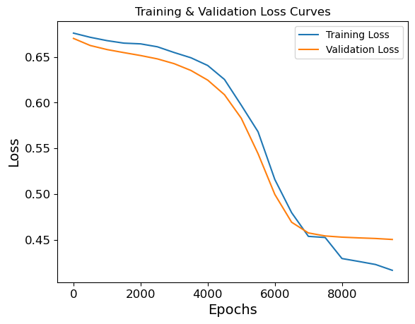
Looks great!
Save this model:
# Create a directory for models
MODEL_PATH = Path('models')
MODEL_PATH.mkdir(parents=True, exist_ok=True)

# Create a model save path
MODEL_NAME = 'pytorch_model.pth'
MODEL_SAVE_PATH = MODEL_PATH / MODEL_NAME

# Save the model state dict
torch.save(obj=model.state_dict(), f=MODEL_SAVE_PATH)
Inference & Submission
Now I’m ready to use the newly trained model to generate predictions for the test set. The first step is to convert the test data to tensors.
Convert test data to tensors:
x_test = torch.tensor(test_proc.values, dtype=torch.float32)

type(x_test)
torch.Tensor
Make predictions on test data:
model.eval()

with torch.inference_mode():
    test_logits = model(x_test).squeeze()
    test_pred = torch.round(torch.sigmoid(test_logits)).int()

test_pred.shape, test_pred[:5]
(torch.Size([418]), tensor([0, 1, 0, 0, 1], dtype=torch.int32))
Convert the predictions to a DataFrame and save to CSV:
submission = test_df['PassengerId'].to_frame()
submission['Survived'] = test_pred

submission.to_csv('model_submission.csv', index=False)
Submit to the Kaggle competition via the API (or you can do this manually on Kaggle’s site):
!kaggle competitions submit -f model_submission.csv -m "PyTorch model submission" -q "titanic"
Successfully submitted to Titanic - Machine Learning from Disaster
And that’s it! Now you’ve seen how to train a simple neural network using PyTorch and used it to generate predictions on a test set.
My best submission scored an accuracy of 77.5% on the Titanic Leaderboard. This is a bit worse than my best score using decision tree algorithms such as random forests (see blog post), which are very effective for structured/tabular data.
Resources
- PyTorch Documentation
- PyTorch Tutorials
- Learn PyTorch for Deep Learning: Zero to Mastery (very detailed tutorials)