Modeling A Single Biological Neuron With Recurrent Architectures
Introduction
This blog post covers my recent work where I trained recurrent neural networks and their variants to learn the inputs/outputs of a single biological neuron.
My motivating goal is to identify neural network architectures that can reproduce the outputs of biological neurons in the human brain. I am particularly interested in models that (a) can be run sequentially, such as recurrent neural networks, (b) are small in size to reduce storage requirements, and (c) are computationally efficient at inference time. Eventually, I’d like to simulate a network of biological neurons co-existing and sharing information processing with a network of artificial “neurons,” each of which is a deep neural network.
Neuroscientists may find such artificial neural networks capable of replicating a biological neuron to be useful in their own work for efficiently simulating a neuron. Current biophysically realistic models that include full morphological and electrical details of neurons are very computationally inefficient, given that they involve numerical integration of thousands of differential equations.
Dataset
To train artificial neural networks, I am using a dataset provided by Beniaguev et al.1 which can be downloaded via Kaggle (more details on the author’s GitHub page). This is a simulated dataset based on a layer 5 cortical pyramidal neuron cell under in-vivo-like conditions, and such neurons are considered to be central to cortical computation due to their nonlinear dendritic operations and extensive dendritic morphology.
This is a diagram illustrating the structural features of a pyramidal neuron, with the dendrites and soma (cell body) in red and the axon in blue:
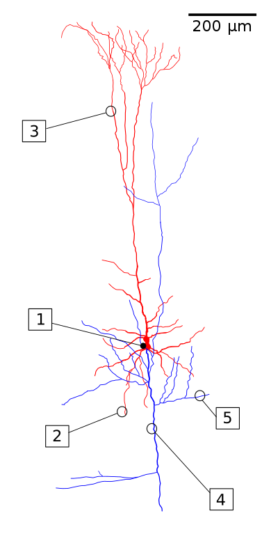
(1) Soma. (2) Basal dendrite. (3) Apical dendrite. (4) Axon. (5) Collateral axon. Image by Fabuio, distributed under the Creative Commons Attribution 4.0 International license.
The provided dataset contains 64 hours of simulation time and is divided into multiple files, each of which contains 128 simulations. Each simulation contains input/output sequences with 6000 timesteps, and each timestep is 1 millisecond long for single spike resolution.
The dataset is split into a training set, validation set, and test set. The training set is the only data that the neural network encounters during training. The evaluation of different models and the selection of best hyperparameters is performed by assessing each model’s performance on the unseen validation set. The test set can be used for reporting purposes on the best-fitting model. The validation and test sets each contain 1280 data samples, and the remaining 35,840 data samples are assigned to the training set, but not all are needed for training to reach convergence.
Data inputs include spike trains from 1278 pre-synaptic neurons. Outputs — which is what the trained models will attempt to predict — include the neuron’s spike output, which is a sequence of 0 and 1 values, as well as the soma’s voltage time series, which is continuous-valued. The neuron’s spike output is very unbalanced and consists of mostly 0 values, and on average has one spike per second of data (i.e., one spike per 1000 timesteps). To address the imbalance, I apply a weight towards the rarer class in the binary cross entropy loss function (more on this in the training details section below).
Recurrent Models
All models explored here are recurrent neural networks (RNNs), including vanilla RNNs as well as their variants such as gated recurrent unit (GRU) and long short-term memory (LSTM). RNNs are a class of artificial neural networks with an internal state (memory) that affects the processing of sequence data.
This diagram shows an RNN in its compressed form (left) and unfolded/unrolled form (right), from Wikipedia:
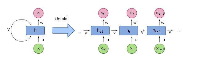
Image by fdeloche, distributed under the Creative Commons Attribution-Share Alike 4.0 International license.
LSTMs were proposed in 1997 by Hochreiter & Schmidhuber2 and improved over the years, typically performing better than RNNs with the ability to detect longer-term patterns in the data. GRUs were proposed more recently in 2014 by Cho et al.3, and they are a simplified version of the LSTM and seem to perform equally well.
LSTMs and GRUs are important for addressing the short-term memory problem in RNNs; as data traverses an RNN, some information is lost at every timestep. In an LSTM cell, the hidden state is split into two states: a short-term state and a long-term state, and the neural network learns what to store in the long-term state and what can be discarded. There is an “input gate” which adds memories, a “forget gate” that deletes memories, and an “output gate” that filters the resulting long-term state. In a GRU cell, there is only a single hidden state, the “forget gate” and “input gate” are merged into a single gate controller, and there is no output gate.
Diagram of an LSTM:
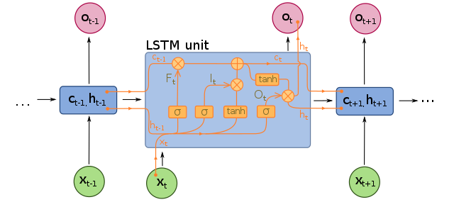
Image by fdeloche, distributed under the Creative Commons Attribution-Share Alike 4.0 International license.
Diagram of a GRU:
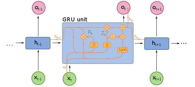
Image by fdeloche, distributed under the Creative Commons Attribution-Share Alike 4.0 International license.
In this work, I explore these recurrent architectures with 3-layer and 6-layer versions. Each layer is defined by the input size (the number of expected features in the input) and the hidden size (the number of features or hidden units in the hidden state). The last layer in the neural network always has a hidden size of 2 because it serves as the output layer and needs to match the number (2) of desired outputs: spike output (0 and 1 values) and soma voltage output (a continuous number). Note that there are no fully-connected layers following the RNN/GRU/LSTM layers. After the output layer, the spike output encounters a sigmoid function and the soma voltage output is multiplied by 100 to scale it in the range of expected values (-100 to +100).
Neural network parameters are initialized as follows: biases are set to zero and weights are initialized according to Xavier/Glorot4 using a uniform distribution, implemented using PyTorch’s torch.nn.init modules.
Experiments
Experiments are performed using PyTorch, which is a Python-based open-source framework for building neural networks (see PyTorch’s Get Started page).
Three model architectures are explored:
- RNN: vanilla recurrent neural network, implemented using PyTorch’s torch.nn.RNN
- GRU: gated recurrent unit, implemented using PyTorch’s torch.nn.GRU
- LSTM: long short-term memory, implemented using PyTorch’s torch.nn.LSTM
as well as six different network sizes (varying the number of layers and the number of hidden units per layer), four different learning rates (0.001, 0.003, 0.006, 0.01) and three different options for a class weight in the loss function (none, 5, and 20). A total of 216 experiments are performed in total.
Models are evaluated based on ROC AUC scores for the neuron’s spike output. The receiver operating characteristic (ROC) is a plot that shows the true positive rate (the fraction of true positives out of all positives) vs. the false positive rate (the fraction of false positives out of all negatives), at various threshold values. The threshold is the discrminating value that separates the two possible classes; in this case, whether the spike output is 0 or 1. Accordingly, the ROC curve demonstrates the model’s performance in a binary classification task. The area under the curve (AUC) calculates the area under the ROC curve so that the information is summarized into a single number. The ROC curve and AUC can be computed using scikit-learn’s roc_curve (documentation) and roc_auc_score (documentation), respectively.
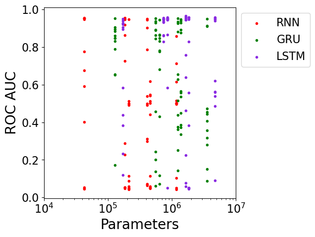
Here are results from all experiments, showing the validation set’s ROC AUC performance vs. the number of parameters in the model with model architectures represented in different colors:
This plot shows the validation set’s ROC AUC performance vs. the number of parameters in the model, only showing the top-performing model for each model configuration (recall that there are 3 model architectures and 6 network sizes for a total of 18 configurations):
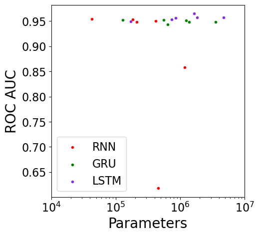
From these plots, it appears that a variety of model architectures and model sizes are able to fit the data reasonably well, despite the model sizes spanning nearly two orders of magnitude from 42,824 to 4,718,624 parameters. It would be interesting to investigate even smaller model sizes to see when performance starts to suffer.
This table summarizes the 10 best-performing experiments, listing their ROC AUC performance on the validation set in descending order:
| Model | Parameters | Layers | Hidden Sizes | Learning Rate | Class Weight | ROC AUC |
|---|---|---|---|---|---|---|
| LSTM | 1,655,840 | 3 | 256-64-2 | 0.010 | 20 | 0.9653 |
| LSTM | 1,655,840 | 3 | 256-64-2 | 0.006 | 20 | 0.9597 |
| LSTM | 1,836,064 | 6 | 256-128-64-32-16-2 | 0.006 | 5 | 0.9576 |
| LSTM | 4,718,624 | 6 | 512-256-128-64-32-2 | 0.003 | None | 0.9573 |
| LSTM | 849,952 | 6 | 128-64-64-64-32-2 | 0.010 | 20 | 0.9569 |
| LSTM | 1,836,064 | 6 | 256-128-64-32-16-2 | 0.003 | 20 | 0.9564 |
| LSTM | 849,952 | 6 | 128-64-64-64-32-2 | 0.006 | 5 | 0.9554 |
| LSTM | 4,718,624 | 6 | 512-256-128-64-32-2 | 0.001 | 5 | 0.9546 |
| RNN | 42,824 | 3 | 32-16-2 | 0.006 | None | 0.9546 |
| LSTM | 1,655,840 | 3 | 256-64-2 | 0.010 | 5 | 0.9539 |
The best-performing experiments are dominated by LSTMs, with only one non-LSTM model — a vanilla RNN — making an appearance. About 53% of LSTM experiments achieved an AUC of at least 0.90, compared to 18% of RNNs and 21% of GRUs.
Models with 3 layers may slightly outperform those with 6 layers, with the former having 37% of experiments achieving an AUC of at least 0.90 and the latter having only 24%.
The top model is a 3-layer LSTM with ~1.7M parameters and an AUC of 0.9653. In comparison, Beniaguev et al.1 achieved an AUC of 0.9911 using a 7-layer temporal convolutional network5 with an estimated ~12 million parameters.
Training Details
All experiments are trained for 200 epochs with a batch size of 32 and a sequence length of 1000 (equivalent to a time window of 1000 milliseconds). A single epoch is defined as iterating through 128 data samples. Since data availability was not an issue, each model did not see the same data sample more than once during training. Note that the sequence length represents the time history of each data sample, and was chosen to be as large as possible without being too computationally expensive.
The learning rate is initialized to 0.001, 0.003, 0.006, or 0.01, and a cosine annealing scheduler is applied so that the learning rate decays over the course of training. It is implemented using PyTorch’s CosineAnnealingLR (documentation), with a T_max of 800 (= 200 epochs * 128 data samples per epoch / batch size) and eta_min of 1e-5.
Two loss functions are implemented. The first loss is the binary cross entropy for the spike output, which is a binary classification task implemented using PyTorch’s BCEWithLogitsLoss (documentation) with a pos_weight applied to positive classes (either no weight, 5, or 20). For example, a pos_weight of 3 means that the loss would act as if the dataset contained 3x as many positive examples. The second loss function is the mean squared error for the soma voltage output, which is a regression task implemented using PyTorch’s MSELoss (documentation) with default parameter values. These two losses are summed together to produce the overall loss.
The optimizer is the AdamW algorithm, implemented as PyTorch’s AdamW (documentation) with weight_decay of 0.01, betas of (0.9, 0.99), and eps of 1e-8.
For a minority of experiments (~12%), the ROC AUC score was unstable during training and did not show steady improvement epoch over epoch. Nearly half of these cases were for vanilla RNN models, with the remainder relatively evenly split between GRUs and LSTMs.
Ideal Threshold
Since the spike output is binary where values can be either 0 or 1, the raw continuous output from the neural network needs to be thresholded at some value to separate the two possible classes. The ideal threshold can be chosen by visually examining the validation set’s ROC curve and selecting a threshold along the curve that maximizes the true positive rate and minimizes the false positive rate. It can also be estimated using the G-Mean score and Youden’s J statistic.
Here are ROC curves for the top-performing RNN, GRU, and LSTM models, with threshold values printed at various points (and corresponding to the colorbar):
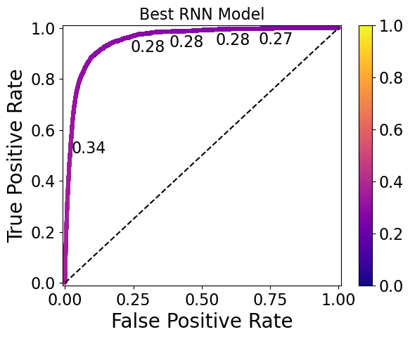
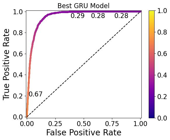
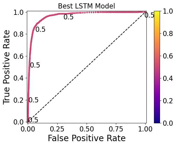
The ideal thresholds for the RNN, GRU, and LSTM models are 0.30, 0.32, and 0.50, respectively. Note that the GRU model has the widest range of thresholds (0.76 to 0.28) displayed on the plot, whereas the RNN model has a narrower range (0.34 to 0.27) and the LSTM has thresholds so similar that they only start to differ at the 5th decimal place.
Models such as the LSTM model shown here require a high level of threshold precision to separate the 0 and 1 classes, and may therefore be undesirable. This should be taken into account in future work during the model evaluation step.
With these ideal thresholds chosen, the true positive rate is about 90% and the false positive rate is about 10-15% for these models.
Future Work
Overall, recurrent architectures such as RNNs, GRUs, and LSTMs are able to successfully fit to training data of a single biological cortical pyramidal neuron. These models are able to predict the neuron’s soma voltage as well as its spike output with reasonable accuracy.
Here are some ideas for future work:
- experiment with smaller model sizes than those explored here, i.e., <40,000 parameters
- optimize a metric that quantifies the spread of raw spike output values (before binarizing into
0and1), since larger spreads require less precision on the exact threshold value - train models using datasets that contain other types of neurons or a network of neurons
-
D. Beniaguev, I. Segev, and M. London, “Single cortical neurons as deep artificial neural networks,” Neuron, vol. 109, no. 17, pp. 2727-2739.e3, Sep. 2021, doi: 10.1016/j.neuron.2021.07.002. ↩︎ ↩︎
-
S. Hochreiter and J. Schmidhuber, “Long Short-Term Memory,” Neural Comput., vol. 9, no. 8, pp. 1735–1780, Nov. 1997, doi: 10.1162/neco.1997.9.8.1735. ↩︎
-
K. Cho et al., “Learning Phrase Representations using RNN Encoder-Decoder for Statistical Machine Translation.” arXiv, Sep. 02, 2014. doi: 10.48550/arXiv.1406.1078. ↩︎
-
X. Glorot and Y. Bengio, “Understanding the difficulty of training deep feedforward neural networks,” in Proceedings of the Thirteenth International Conference on Artificial Intelligence and Statistics, JMLR Workshop and Conference Proceedings, Mar. 2010, pp. 249–256. ↩︎
-
S. Bai, J. Z. Kolter, and V. Koltun, “An Empirical Evaluation of Generic Convolutional and Recurrent Networks for Sequence Modeling.” arXiv, Apr. 19, 2018. doi: 10.48550/arXiv.1803.01271. ↩︎